Perth’s freeway network has undergone significant changes in recent years. One of the more controversial upgrades is the Smart Freeways project; a modification which aims to improve travel times of commuters from the city’s outer suburbs heading toward the center. This system has been implemented on both the Kwinana Freeway Northbound and the Mitchell Freeway Southbound, managing traffic flow primarily through digital speed-limit gantries and on-ramp metering. On the Mitchell South, travel times during the morning peak have been reduced by up to seven minutes for trips from Hester Avenue, Clarkson to Vincent Street, Leederville (Main Roads, 2025). Road users further north
enjoy these improved speeds as they spend a majority of their journey on the freeway mainline. However, commuters closer to the city are more affected by ramp-metering, since a smaller proportion of their trip occurs on the freeway itself. As a result, some drivers have reported their morning commute times more than doubling in length (ABC, 2025).
Ramp Signals - Main Roads (2025)
This study will focus on the interchange between Reid Highway and the Mitchell Freeway southbound. This is a critical link in Perth’s north-west suburbs, as it represents the only highway–freeway interchange in the area and is important in the movement of both people and goods each day.
Reid Hwy / Mitchell Fwy Interchange - Google Maps (2022)
The aim of this study is to determine whether the reported improvements in mainline travel times are offset by increased queuing times for users of this interchange. This will be evaluated by developing a queuing model based on historical traffic data, allowing a comparison of the time spent waiting to enter the freeway with previously reported savings. We will additionally perform parameter optimisation to minimise timing while maintaining stability of the system. For this, it is important to understand the background of stability for a model.
A queuing system with \(c\) lanes is stable (i.e. has a controllable load) if its utilisation rate \(\rho = \frac{\lambda}{c \times \mu}\) is less than \(1\), where \(\lambda\) and \(\mu\) refer to the mean arrival and departure rates respectively (Righini, 2020). In terms of ramp-metering, this utilisation rate is typically maintained in a range below capacity as a means of risk aversion, or avoiding a total breakdown of the queue system (Levinson, 2021).
Methodology
Main Roads have a large online repository of traffic volume measurements from 2013 to the present day. Each entry is a 15-minute interval which can be accessed for any road segment using its unique MLinkID. We can filter for the on-ramp of interest using its ID 5725:
Here, ‘Volume’ refers to the count of vehicles, and ‘TravelTimeMinutes’ the average time to travel that particular road segment.
In order to construct a queuing model, we can use this dataset to simulate the incoming volume of traffic during the morning peak. Typically, this model would be formed on the Poisson distribution because of its memoryless property and ease of implementation.
The memoryless property of the Poisson process implies that the probability of future events is completely independent of the past. This is because the process is unable to ‘mathematically determine’ the time that has passed since the previous event.
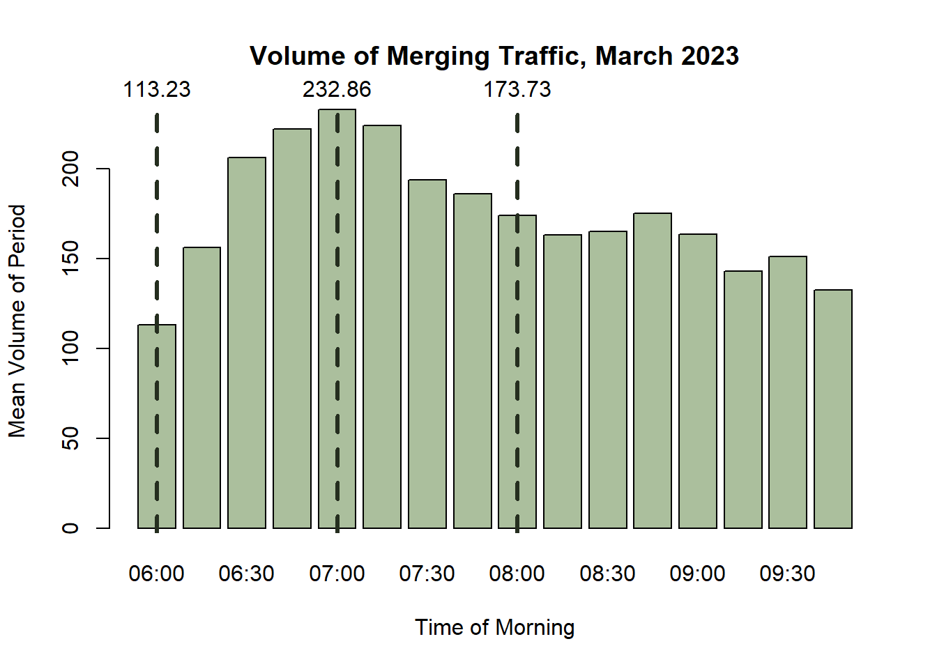
However, a Poisson distribution assumes an equal mean and variance, so it’s important that verify this assumption. To visualise, let’s filter the above dataset to account for weekdays, the peak hours, and without public holidays (eg 06/03/23 : Labour Day), plotting the volume for each 15-minute interval:
The volume of traffic entering the freeway varies heavily over the course of the morning. In order to optimise for the local demand peak, consider a piecewise model. Simulations that account for the minimum, maximum and mean volume each morning will be constructed, correlating to the times 6am, 7am and approximately 8am. If instead we averaged the entire peak, we would fail to capture actual demand. This way, we can simply extrapolate a best and worst case through as many timesteps as needed (rather than trying to represent the whole morning).
We’ll focus on the 6:00-6:15am interval for now:
              Mean Variance
6am (min) 113.2273  161.803
This is an overdispersed dataset where the variance of volume is considerably higher than its mean. This is true throughout the entire dataset, meaning a Poisson distribution would be unsuitable as we do not satisfy the assumption of equidispersion. In order to provide a better fit, we can consider a Negative Binomial where both a mean and a size parameter (which represents the clustering phenonmenon) can be selected.
Whilst a Negative Binomial relaxes the memoryless assumption, we must still assume independence of each arrival event. In reality, this is not the case because travelling vehicles tend to congregate in groups called ‘platoons’. Because our on-ramp is preceded by a signalised intersection, we would certainly see vehicles arriving based on it’s signal timing. As a result, the final model may underestimate variability in arrival patterns and associated queue timing.
However, because we are only considering the traffic volume at a single point in time (and extrapolating many timesteps from it), we can somewhat relax this assumption as well.
We can calculate the size parameter \(r\) for a Negative Binomial as follows:
\[r = \frac{\mu^2}{\sigma^2 - \mu}\]
To see the improvement in fit, let’s simulate a Poisson and a Negative Binomial with these parameters and compare with the original dataset.
The Negative Binomial is a much better fit to the original dataset. However, a new concern arises: for the purpose of simulation, we wish to simulate vehicle-counts on a per-minute basis. This will help to increase the granularity of our queuing time results beyond the 15-minute intervals provided in the dataset. One possible solution ( Method 1 ) is to simply divide the volume data by \(15\) and fit a new model. If we consider this case, our mean will scale by a factor of \(\frac{1}{15}\), and the variance by a factor of \(\frac{1}{15^2}\):
1-min Model Parameters (Method 1)
                 Mean  Variance      Size
Vehicles/min 7.548485 0.7191246 -8.343333
Since this is now underdispersed, a Negative Binomial will no longer fit (hence the negative size). It remains unbiased, but erases so much of the original variance that it is completely irrelevant. An alternative solution (Method 2) that maintains our original variation is to use the divisible property of the Negative Binomial. We first form the model, then scale its parameters to maintain a dispersion that remains in proportion to the new, lower mean.
This occurs because the Negative Binomial is formed as a Compound Poisson (Siegrist, 2022), so if \(X=X_1 + X_2 +...+X_n \sim NBinom(k, p)\) then we can model each \(X_i\) as \(NBinom(\frac{k}{n}, p)\) with the same probability \(p\). Extrapolating this \((_{successes}, \space _{probability})\) form to the \((_{mean}, \space _{size})\) form yields the parameters \((\frac{\mu}{n}, \space \frac{r}{n})\).
Although this is a valid process for the Negative Binomial, we have to make an additional assumption that the volume in each 15 minute interval is uniform. Because of the signalised intersection preceeding the on-ramp, we would inevitably see heavy platoons or ‘bursts’ forming each couple of minutes. Because our simulation erases this variability, it means that the wait-times we find are still likely to underestimate reality.
1-min Model Parameter Comparison (Methods 1 and 2)
In terms of release rates, on-ramp metering historically operates on deterministic parameters. This means that a fixed number of vehicles are released per time-unit, assuming that vehicles do not run the stop phase. Modern-day systems implement a more dynamic rate, determined live from mainline traffic volume and speed (Dot.gov, 2000). However, these still remain inherently deterministic because given a set of conditions, there is mathematical reasoning behind the release rate, not randomness.
Therefore, as our model will not account for changes in mainline flow, we will use a simple deterministic release rate.
Model Implementation and Results
To evaluate the impact of ramp-metering on queue lengths and wait-times, a custom queuing simulation was developed. Whilst standard models, such as an M/D/c, are capable of estimating steady-state averages, they cannot easily accommodate the overdispersed Negative Binomial arrival patterns or allow for sub-15 minute granularity. Hence, the most logical approach was to develop a discrete-event simulation that evaluates queues based on a per-minute basis.
The most logical choice was to develop onRampSimulation, as a G/D/c queue using the following logic:
During initialisation, the function sets up empty vectors to track incoming and outgoing volume, queue length, and both average and individual wait times across all time steps. A fixed random seed is used in the function top employ the CRN (Common Random Numbers) variance reduction technique which will allow us to compare different departure rates \(\mu\) against the exact same arrival sequence without random noise obscuring the comparison.
We employ stochastic arrivals at each timestep using the Negative Binomial Distribution based on specific \(\mu\) and size parameters calculated from the relevant Main Roads data set. These vehicles are, in a nutshell, stamped, and added to the back of the queue.
Whilst it is known that the ramps function on a deterministic release rate, when simulating at a per-minute interval, the release rate could potentially become fractional (i.e., 8.5 vehicles per minute). As logic prevails, it is not possible to have a fractional component of a vehicle, the simulation has been designed around this potential break-point and is able to pass fractional components onto the next release by using a \(\text{carry}\). This slightly deviates from a standard G/D/c model, but this trade-off is worth forcing for a more realistic discrete vehicle model.
It may have been made obvious at this stage that there is a deviation from the G/D/c approach as the designed simulation does not have a strictly deterministic system. The reason for this is due to the carry. The carry creates deviation in the release of vehicles, as an example, if it is calculated that 3.5 cars are released in 2 iterations, the first iteration will release 3 cars and the second will release 4 cars, and this release pattern is not entirely deterministic. We have decided to trade the strictly deterministic approach for one that is more realistic which is arguably more useful to the model.
The model finally is able to release the allocated number of vehicles (or entire queue if the queue < release rate). Because we stamped the vehicles with an arrival time, the wait time for each departing vehicle is simply calculated as \(\text{Current Time-step - Arrival Time-step}\)
onRampSimulation <-function(steps, alambda, asize, rmu, c) {set.seed(1234) queue <-c() # storage for vehicles currently in queue incoming <-numeric(steps) # track count of vehicles arrived outgoing <-numeric(steps) # track count of vehicles released wlength <-numeric(steps) # track length of queue in each timestep wtimesavg <-numeric(steps) # track AVERAGE waiting times of vehicles released in a timestep wtimesall <-c() # track INDIVIDUAL waiting times of vehicles released in a timestep# need to incorporate a carry because vehicles are individisble.# if the release rate is fractional,# we can 'pass' off the next vehicle to the following timestep carry <-0for (i in1:steps) {# calculate arrivals arate <-rnbinom(1, size=asize, mu=alambda) queue <-c(queue, rep(i, arate)) incoming[i] <- arate# calculate departures fracrrate <- rmu * c + carry rrate <-floor(fracrrate) carry <- fracrrate - rrate released <-min(length(queue), rrate) outgoing[i] <- released# release cars and track wait timesif (released >0) { rtimes <- i - queue[1:released] wtimesavg[i] <-mean(rtimes) wtimesall <-c(wtimesall, rtimes) queue <- queue[-(1:released)] } else { wtimesavg[i] <-0 } wlength[i] <-length(queue) }return(list(incoming = incoming,outgoing = outgoing,wtimesavg = wtimesavg,wtimesall = wtimesall,wlength = wlength) )}
Part 1 - Sensitivity Analysis
For each model we have developed, consider the critical point where the utilisation parameter \(\rho\) is exactly one. Rearranging in terms of the release rate, we find \(\mu = \frac{\lambda}{1 \times c}\) whichs allows us to determine the largest timing possible for each system to remain stable. As 2 lanes are present at the Reid Highway on-ramp, we set \(c=2\) and form three G/D/2 queues with the following parameters:
Arrival and departure parameters for each model case
                      Best     Worst   Average
Mean Arrival Rate 7.548485 15.524242 11.581818
Departure Rate    3.774242  7.762121  5.790909
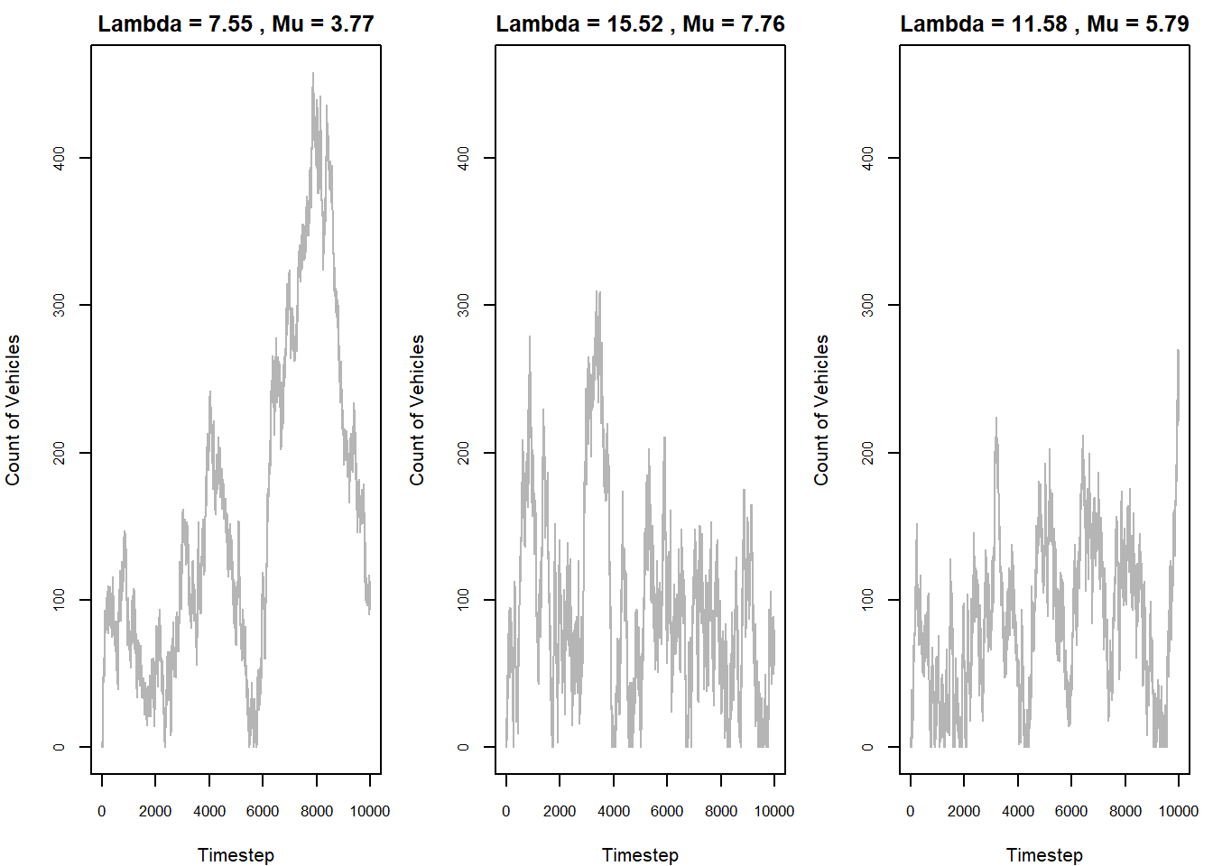
We can start by running the above simulation for the minimum (best, 6am), maximum (worst, 7am) and mean (average, 8am) models for a long-term scenario (\(10000\) timesteps). Here, the Law of Large Numbers applies making the estimates highly stable.
Best, Worst and Average Case Simulations (at critical points)
[1] "Maximum length: 458"
While in all cases there is theoretical stability (i.e. the models will all return to 0), we can see that a utilisation rate of exactly \(1\) is completely unreasonable in a real-world scenario. The 6am (leftmost) model particularly balloons to a queue of over 400 vehicles long, with the others reaching more than 200 vehicles each. In reality, a utilisation rate closer to 90% is generally maintained to balance throughput with wait times.
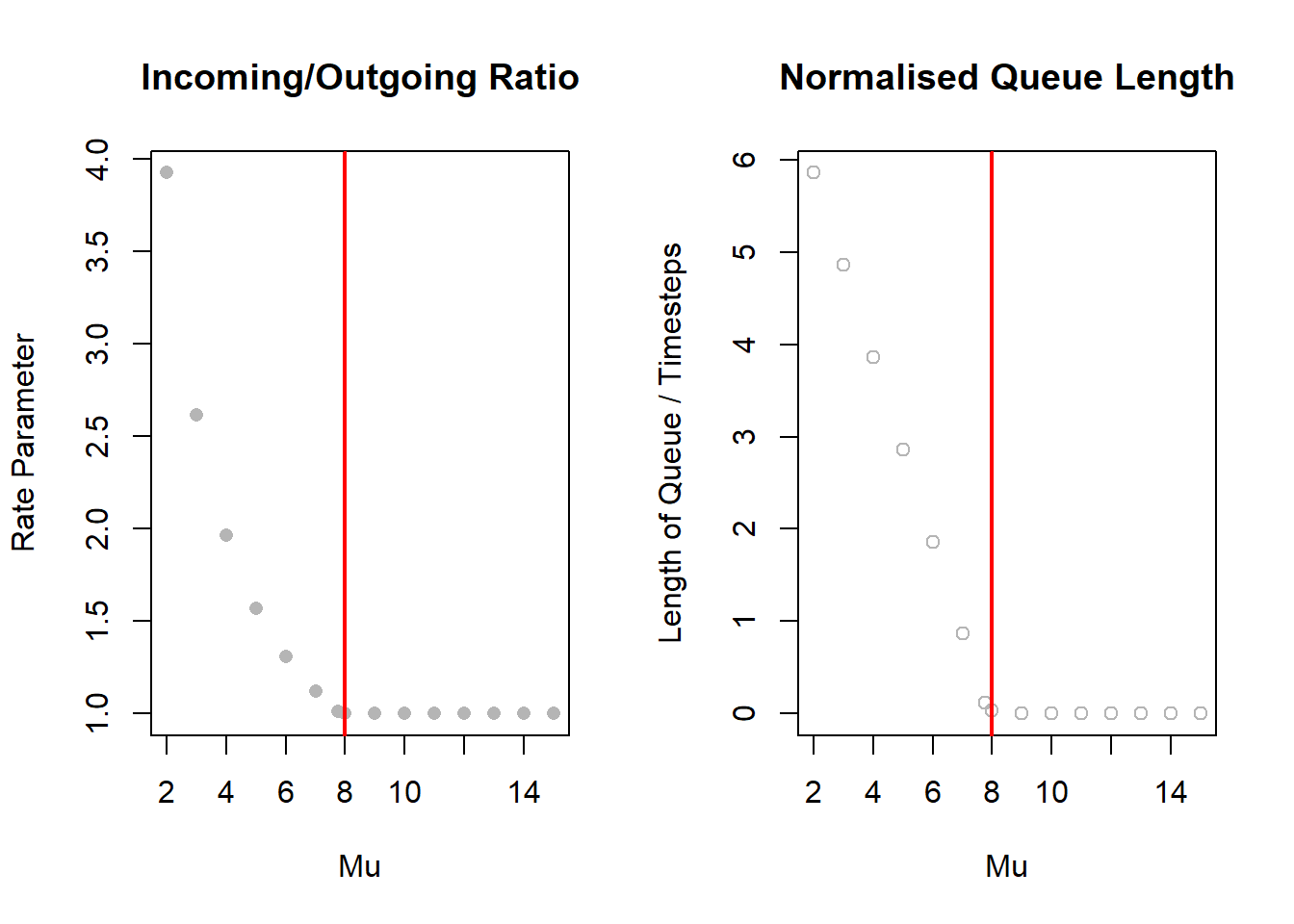
Focusing on the 7am (center) scenario, we can reaffirm the visualisions through a plot of the ratio of net arrival-to-depature counts for a series of release rates \(\mu\). This ratio can be \(1\) at minimum as we can only have as many vehicles departing as there were vehicles that have arrived in the first place. However, when the system is past stability this ratio is unbounded.
[1] "Recall that the incoming rate is 15.52 with a critical Mu of 7.76"
For \(\mu \geq 8\), this ratio is clamped at one as was expected. However, for \(\mu < 8\) there is an unbounded hyperbolic growth in the ratio of incoming-to-outgoing vehicles. A larger ratio means there are consistently more vehicles arriving than the system can output, and so if this is above one total breakdown will occur.
This suggests the system is very sensitive to changes past the critical threshold while \(\rho\geq1\). A small decrease in \(\mu\) has a proportionally large, non-linear increase in the ratio parameter.
To investigate further, we can shift focus to the normalised queue length plot on the right. Here, notice the linear shape past the same critical point as \(\mu < 8\). We can define this region by the line:
We find a slope of \(-0.999 \approx -1\), suggesting that for every unit increase in \(\mu\) getting closer to the critical value \(\mu=8\), we lose a unit of length in the queue. So while the ratio parameter seems to grow exponentially, the relationship between the resulting length of the queue for a given release rate \(\mu\) is linear. Therefore, while small changes in \(\mu\) impacts the queue length significantly, the queue will break down in a very predictable and manageable way.
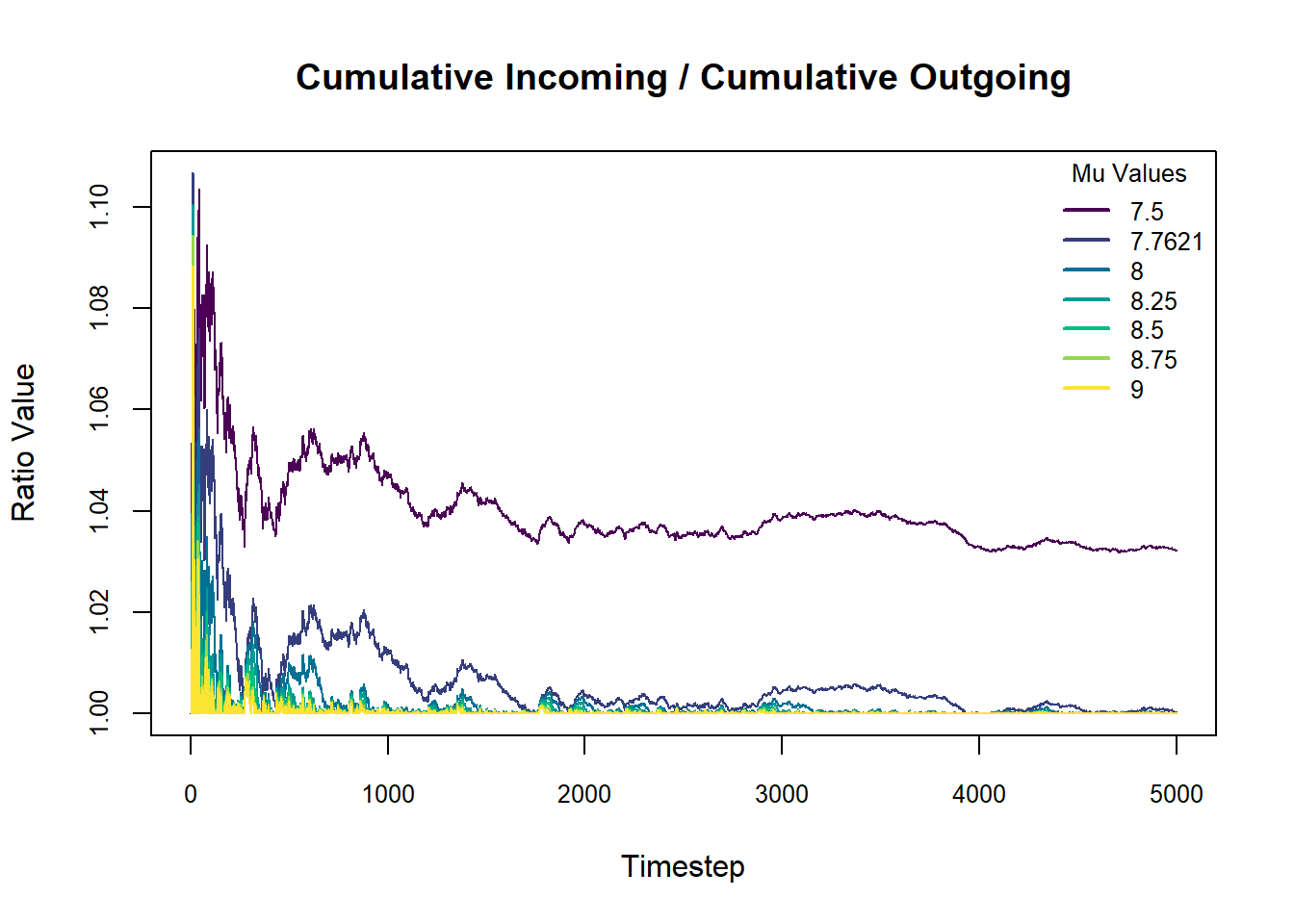
Let’s now shift focus to the sensitivity of the system while in stability, or when \(\rho < 1\).
As before, we need this to trend near \(1.00\) for long-term timesteps, otherwise there are consistently more vehicles arriving than leaving. This seems to occur for all but the smallest \(\mu\) value which is clearly disjoint from the rest. We can therefore say that for \(\mu \geq 7.76\), the critical threshold, the lines appear to converge and return back to \(1.00\).
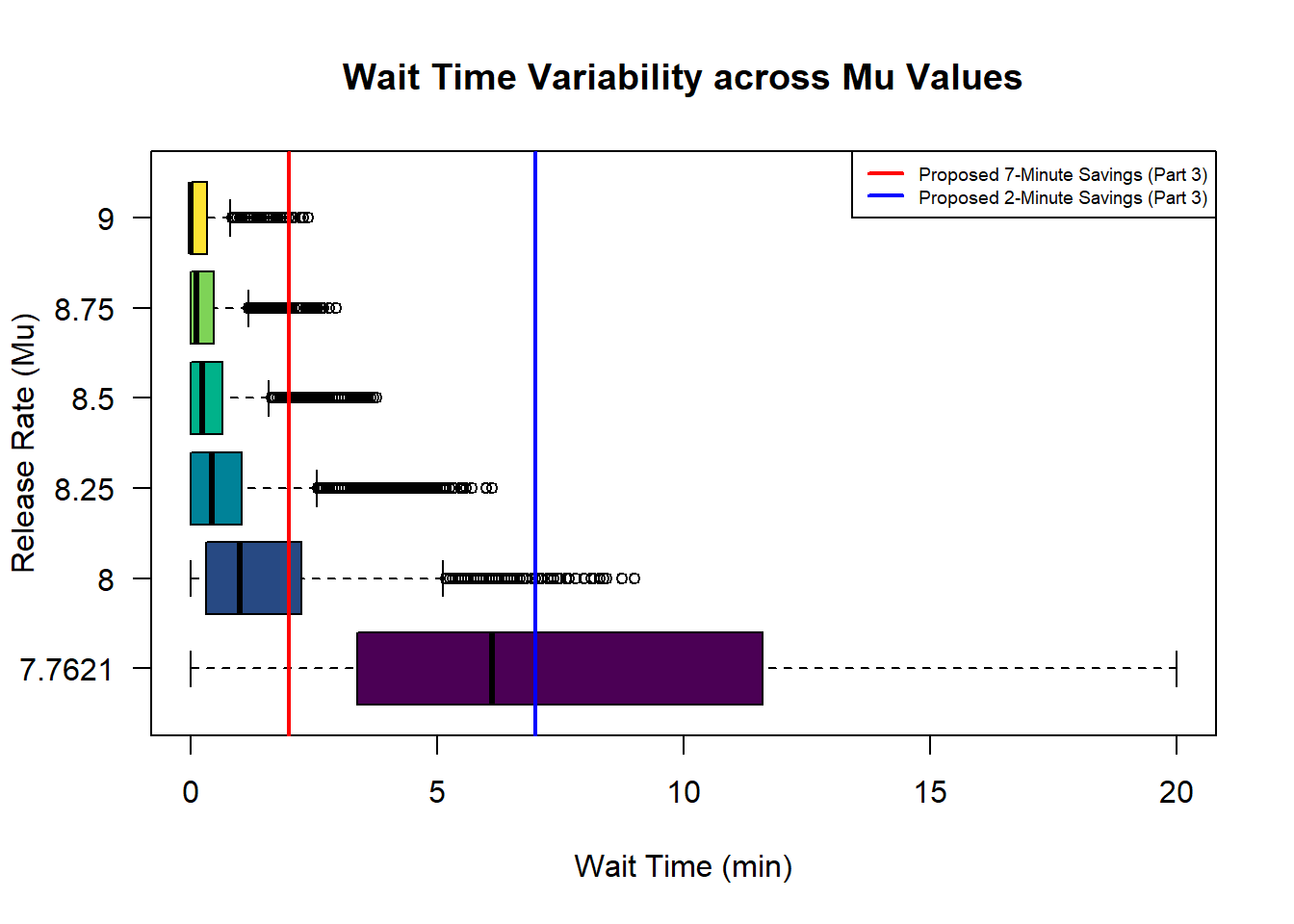
We can also visualise the wait-times of simulated users in a series of boxplots:
This is a plot of average wait-times for each timestep, allowing us to achieve sub-1-minute resolution. This slighly reduces the maximum wait-times seen but greatly aides the visualisation.
There is a clear exponential growth for the boxplots as \(\mu \rightarrow 8\), or in other terms \(\rho \rightarrow 1\):
the median wait time for vehicles increases;
it’s IQR widens; so we have more uncertainty if quoting a given mean
the whiskers grow far longer; so outlier vehicles will notice a disproportionally extreme increase in wait time
A reasonable choice that seems to fit the predictable side of every-day traffic would be \(\mu=8.00\).
summary(plotlist$"8")
   Min. 1st Qu.  Median    Mean 3rd Qu.    Max.
 0.0000  0.3125  1.0000  1.5904  2.2500  9.0000
Here, 75% of drivers are waiting under \(2.25\) minutes with an overall median of \(1\) minute. However, notice the maximum wait-time of \(9\) minutes. A wait of this length is considered completely unreasonable, so if we instead account for these outlier vehicles (or for more ‘extreme’ conditions), it takes until \(\mu = 8.5\) before the maximum wait drops past \(5\) minutes.
   Min. 1st Qu.  Median    Mean 3rd Qu.    Max.
 0.0000  0.0000  0.2353  0.4717  0.6471  3.7647
summary(plotlist$"8") #97.0% utilisation
   Min. 1st Qu.  Median    Mean 3rd Qu.    Max.
 0.0000  0.3125  1.0000  1.5904  2.2500  9.0000
At the more conservative utilisation rate, drivers will have a maximum wait time of \(3.76\) minutes. However, notice that the average wait-time is under \(30\) seconds. The purpose of ramp-metering is to average out the ‘platoons’ of incoming volume so that the mainline sees a smooth and predictable flow. This scenario raises the question whether this wait would be sufficient to eliminate the intense burstiness enough not to impact the mainline flow. This is outside of the scope of this study, but is something that must be considered.
Moving on, consider above how all the boxplots are heavily right-skewed, demonstrating that regardless of our maximum wait-time, a majority of commuters will not be impacted by a changing \(\mu\). So, while the median wait-time is decreasing, it is at a far slower rate than the extreme change we see in the outliers.
We can therefore split the sensitivity of a stable system into two distinctions:
The \(50th\) and \(75th\) percentiles (wait-times for the majority of drivers) seem relatively insensitive to changes in \(\mu\);
The outlier wait-times remain highly sensitive to changes in \(\mu\)
Once below about \(95\%\) utilisation, there is only a minimal improvement to wait-times for the \(50th\) and \(75th\) percentiles even for a large change in the release rate. This means that it is critical to find a \(\mu\) that balances both a consistent and restrictive release of vehicles without breaking down. A system that would function best here is one with live feedback - dynamically adjusting its \(\mu\) based on a live wait-time distribution.
Part 2 - Transient Response
Another important regard is to understand how the queuing system responds to a sudden change in the vehicle arrival pattern. For this we need to develop a new function, identical but including:
A parameter for vehicle injection (discrete surge) at timestep P
A parameter for a model shift (changing to a new arrival rate and size) at timestep Q
A maximum queue length before a temporary third lane is opened
Let’s first consider a more common scenario. This model will demonstrate the effect of an unexpectedly heavy light-phase, and will use the parameters:
\(91.3\%\) utilisation rate
6am parameters
20 vehicle injection at \(T=5\)
We can use a plot of cumulative arrival and departure counts to see how the system recovers after this slug.
The two arrival and departure lines must converge at all time for a stable system. However long it takes for this equilibrium to reoccur after our step change is a measure of recovery time. Therefore, it takes approximately 13 minutes for the on-ramp to clear the slug and ‘catch-up’ with its regular input. This represents a quantifiable and realistic way that the system would react to a sudden inflow of vehicles.
summary(sim$wtimesavg)
   Min. 1st Qu.  Median    Mean 3rd Qu.    Max.
 0.0000  0.0000  0.2500  0.6361  1.2153  2.3333
Road users are only mildly impacted with \(75\%\) of drivers waiting under 1.21-minutes, and the maximum wait remaining under three.
Let’s consider a more extreme scenario, where an accident has occurred at the intersection preceding the on-ramp. We’ll assume it takes 10-minutes for the accident to clear, causing a queue of vehicles to form behind.
Once cleared, all vehicles are assumed to enter the on-ramp simultaneously, and traffic resumes as normal (i.e. like before, this incident occurs on-top of regular traffic flow).
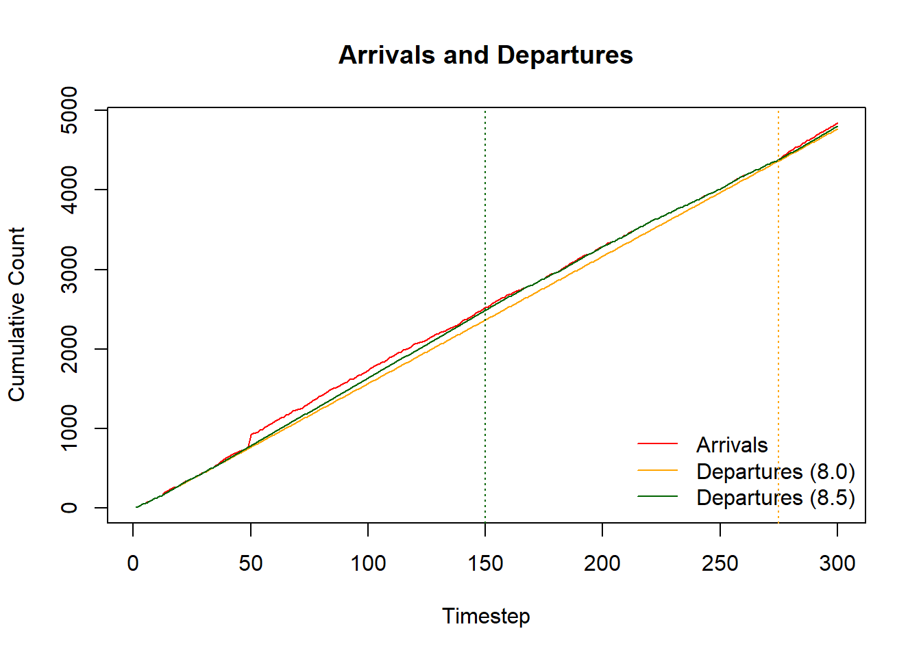
Vehicle injection comparison at timestep 50
The conservative model (\(\mu = 8.5\), \(\rho=91.3\%\)) recovers somewhat quickly, with its departure slope increasing until it meets the arrivals near \(T=150\). Since the system is comfortably under capacity, if more vehicles are present it has the ability to increase its output to match. On the other hand, the everyday model (\(\mu = 8.0\), \(\rho=97.1\%\)) converges closer \(T=275\), making it \(\frac{100}{225}\approx40\%\) slower. Regardless, both models still take over an 90-minutes to ‘catch-up’ to their regular input. This again highlights the importance of feedback; a system that would perform best here is one that can comfortably restrict traffic flow under regular conditions, but increase its release rate in reaction to longer queues.
summary(sim2$wtimesavg) # 91.3% utilisation
   Min. 1st Qu.  Median    Mean 3rd Qu.    Max.
  0.000   0.000   1.000   2.168   3.588   8.000
summary(sim1$wtimesavg) # 97.1% utiisation
   Min. 1st Qu.  Median    Mean 3rd Qu.    Max.
  0.000   3.000   7.281   6.284   9.641  11.438
Like before, we can see that the wait-times of road users are still not greatly impacted. Even in a more extreme scenario, although it may take some time for the system to ‘catch-up’, road users do not actually experience this as a significant increase in their individual wait-times.
Part 3 - Overall System Impact
Main Roads has a proposed 7-minute improvement in Southbound travel times following the implementation of Smart Freeways. This is calculated from Hester Avenue (Clarkson) to Vincent Street (Leederville), but there are no defined figures from Reid Highway specifically.
We can estimate this through the proportion of lengths:
Hester Avenue to Reid Highway is approx. 22km
Reid Highway to Vincent Street is approx. 10km
If we assume that time improvements are uniform across the freeway, we can equate a conservative saving of 2 minutes on the Southern segment. For the previous models, we can estimate the net improvement/detriment to commuters by comparing the distribution of on-ramp wait-times with this value.
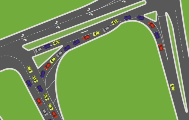
Since this we are considering the system as a whole here, let’s also expand to moderate spillback. Spillback occurs when a signal provides insufficient capacity, forming a queue that affects and blocks throughput of neighbouring intersections. We first need to find the maximum capacity of the road segment:
Example of Spillback - Main Roads (2025)
According to Google Earth, the length of road preceding the on-ramp signal is:
Single lane: 330m, and
Double lane: 120m
We can also source an effective 8.5m length for a queued passenger vehicle (Main Roads, 2018), accounting for both the length of the vehicle and a gap infront. This leads to a total capacity of \(\frac{330+120 \times 2}{8.5}\approx67\) vehicles before spillback occurs.
Consider two models with the following parameters:
\(91.3\%\) and \(97.1\%\) utilisation rates
Arrivals and departures corresponding to 8am
Opening a temporary, third lane when reaching 70% spillback of the network
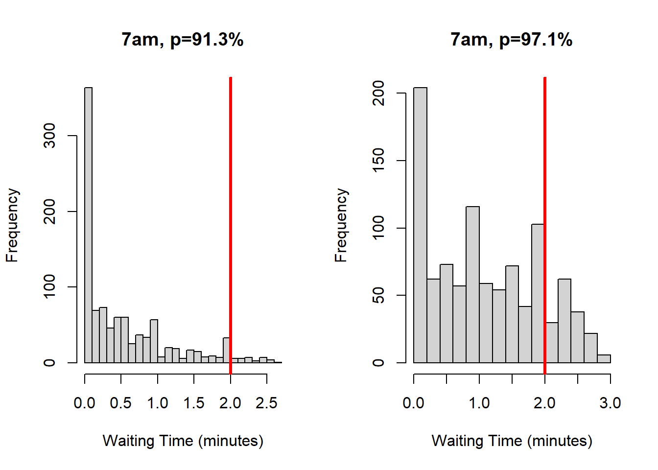
threshold <-67*0.7# open temp lane at 70% capacitypar(mfrow =c(1, 2))# testing 91.3% utilisationsim88 <-onRampTransientSimulation(1000, smu7, ssize7, rmu7 /0.913,threshold = threshold)hist(sim88$wtimesavg, main ="7am, p=91.3%", xlab="Waiting Time (minutes)", breaks =20)abline(v =2, lwd =3, col="red")# testing 97.1% utilisationsim94 <-onRampTransientSimulation(1000, smu7, ssize7, rmu7 /0.971,threshold = threshold)hist(sim94$wtimesavg, main ="7am, p=97.1%", xlab="Waiting Time (minutes)", breaks =20)abline(v =2, lwd =3, col="red")
# Confirming spillback has not occured (<67)data.frame(maximum =67,conservative =max(sim88$wlength),everday =max(sim94$wlength))
  maximum conservative everday
1      67           45      65
A \(97.1\%\) utilisation rate is in theory fine, but the system would suffer a total breakdown in the event that a single slow truck or minor vehicle surge occurs, pushing the system over its capacity. This entails that a system with \(91.3\%\) utilisation would serve better to reduce the chance for spillback to occur. This is due to the fact that with the higher utilisation model, there is only a 2 vehicle buffer, whereas with the \(91.3\%\) model, the buffer would be \(67 - 0.913\times67= 5.829 \approx 5\) vehicles.
The distribution of wait times for both utilisation rates appears somewhat exponential. For \(\rho =97.1\%\) however, we see a stronger uniformity on the tail end. This means that a greater proportion of users are waiting longer at the on-ramp. To quantitatively define this, consider a test for the proportion of vehicles with a 2-minute-or-longer wait at the on-ramp, whose net-travel time across the Southbound Freeway has increased:
\[
H_0 = p \leq p_o\
\]
\[
H_a = p > p_o
\]
For a threshold of 10% of drivers with a net increase, (i.e. \(p_o=0.1\)) and at 95% confidence, see:
For a utilisation rate of \(91.3\%\), we yield an extremely high p-value – we cannot reject the null and so the proportion of drivers seeing an overall increase in journey time is insignificant compared to \(10\%\). Alternatively, for a \(97.1\%\) utilisation rate we see a p-value much lower than 0.05. Here, we are \(95\%\) confident that the true proportion of drivers waiting more than 2-minutes is at least \(13.9\%\), a significant result.
So, at the higher every-day utilisation rate, the system does have a statistically significant proportion of road users whose overall journey time on the freeway has increased.
summary(sim94$wtimesavg)
   Min. 1st Qu.  Median    Mean 3rd Qu.    Max.
  0.000   0.375   1.000   1.107   1.812   3.000
mean(sim94$wtimesavg <2)
[1] 0.784
However, because we incorporate feedback, the new maximum wait-time is only \(3\) minute (down from \(9\)). In this situation, \(78.4\%\) (a majority) of drivers will still see a net improvement in their travel time when heading towards the city. Due to the inherent variation of traffic flow, it is not reasonable for every driver to individually see a net improvement in their travel time from this on-ramp. For some, and most, road users it is – but not all.
Conclusion
Overall, a great majority of road users will see a benefit from Smart Freeways. We have seen that the third quantile of wait-times is generally insensitive to changes in release rates as long as stability is maintained. It typically remains under 2 minutes, meaning that \(75\%\) of drivers will either not be affected at all, or will remain to see a net improvement in their travel times. Rather, what does seem to grow exponentially are the outlier wait-times. Therefore, this study does not invalidate drivers who have experienced unreasonable journeys on the Smart Freeways system. We have seen that this is certainly possible, with wait-times pushing above 9-minutes in our earlier every-day models. However, when feedback is incorporated, it is possible to both sufficiently restrict traffic while keeping maximum wait-times acceptable even in the event of a surge. An appropriate utilisation range appears to be in the range \((91.3\%, 97.1\%)\), with values on the higher end achievable by incorporating feedback and a temporary third-lane. Of course, these findings are only valuable for the Mitchell Southbound on-ramp via Reid Highway.
The largest limitation of the study is that it did not deeply consider the influence of released vehicles on the freeway itself. After all, the very purpose of ramp-metering is to smooth out ‘platoons’ of vehicles entering the mainline. Therefore, its possible that in a pursuit of smaller wait-times, we adjusted the release rate in a way that diminishes this important purpose. This limitation is in conjunction with the resolution of the study. While efforts were made to increase granularity from 15-minutes to one, it would be useful to zoom in even further. Perhaps we could measure the system’s response to the arrival of vehicles over a single light phase – allowing us to judge how it averages out a single ‘platoon’. However, this would require more detailed measurements of the light phases and cycles of the preceding intersection.
The simulation also only measures a single point in time, extrapolated as many timesteps as needed. In the future, it could be expanded to consider the entire course of the morning rush, with the release rate dynamically adjusting based on arrival patterns.
Nonetheless, the study remains strong at highlighting the overall, large-scale impact of ramp-metering on road users. Given an appropriate utilisation rate, even significant step-changes do not greatly impact the wait-time distribution of vehicles. Therefore, for the majority of road users, Smart Freeways is a system which shows great potential given that it is appropriately optimised and incorporates feedback.
References
2025 Annual Report | Main Roads Western Australia. (2025). Wa.gov.au; Main Roads Western Australia.
Righini, G. (2022). Introduction Probability distributions Birth-and-death process Results for some queuing systems Queuing systems design Queuing theory.
.gif)